6.Tutorial
A case by case tutorial.
| Tutorial ID | Description |
|---|---|
| 6-1.Public data | How to analyze a public data with GEO accession number. |
| 6-2.Public data | How to analyze a list of public data with a text file containing the list of GEO accession numbers. |
| 6-3.Private data | How to setup Private table for user's data. |
| 6-4.Private data | How to setup Private table when you have multiple files for a single sample: Multi-lane. |
| 6-5.Peak Calling | How to identify peaks using Peak Calling with the output. |
| 6-6.Graph | How to draw Graph with the output. |
| 6-7.IGV | How to explore genome using IGV with the output. |
| 6-8.Custom adapter sequence | how to use a custom adapter sequence generated by ownself. |
| 6-9.Motif analysis | how to discover de novo and known motif using the output file of Octopus-toolkit. |
6-1.Public data (Single GSE/GSM)
Note
6-1.Public data (Single GSE/GSM) describes how to process publicly available data by entering a single GEO accession number.
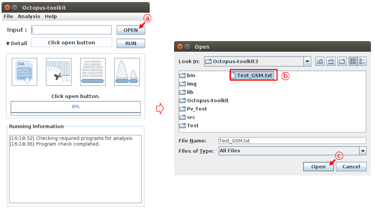
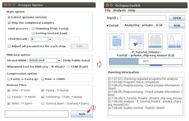
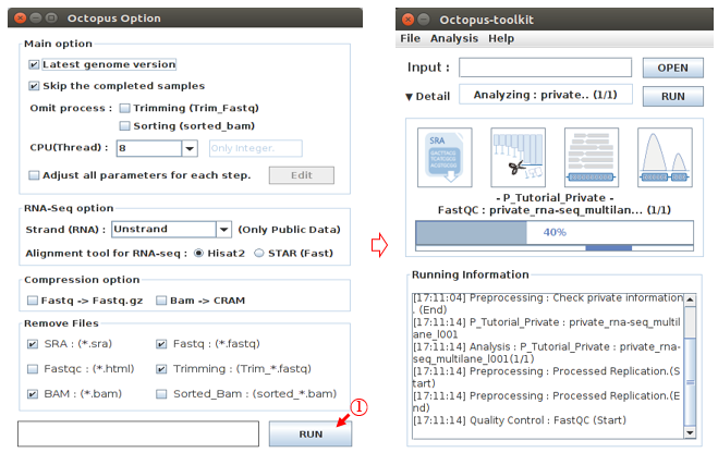
Analyzing published data is a simple process. Enter a GEO accession number in the input text area. Then click the Run button and Octopus-toolkit option window will appear. In the Option window, set the parameters for the analysis and click the RUN button to begin the analysis.
GEO accession number: GSE48685 (ChIP-Seq:10, RNA-Seq:1)
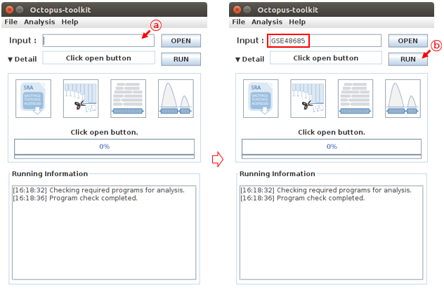
A: Enter GSE48685 in the input text area.B: Click the Run button
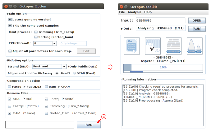
C: Select the options to analyze and click the Run button. (Option : Defalut)
Finally, Octopus-toolkit will automatically download raw files in the GSE48685 ftp directory and subsequenty analyze the data. The output will be stored in a specified directory. No other action is required.
6-2.Public data (Multi GSE/GSM)
Note
6-2.Public data (Multi GSE/GSM) describes how to sequentially analyze a set of public data (a list of GSE accession numbers).
You may want to analyze samples (GSM) in a study (GSE) with several other studies (GSEs) altogether. In this case, you need to create a text file containing GSM ids for samples and GSE ids for studies.
An example is shown below. (example.list)
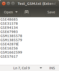
Then, click the OPEN button and select the list file you prepared.
A: Click the Open buttonB: Select the GEO accession number list file.C: Click the Open button
Then, click the RUN button. Octopus-toolkit option window will appear. In the Option window, set the parameters for the analysis and click the RUN button to begin the analysis.
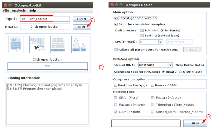
D: Click the RUN buttonE: Select the options to analyze and click the RUN button. (Option : Defalut)
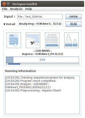
Finally, Octopus-toolkit will automatically analyze the list of data. Sit back and relax until the results are out.
6-3.Private data (Basic)
Note
6-3.Private data (Basic) describes how to analyze your own data using the same analysis pipeline for the public data.
Let’s assume that you have the following data.
| NO | File name | Genome | Seq Type | SE or PE | Strand |
|---|---|---|---|---|---|
| 1 | Private_ChIP-Seq_Mouse.fastq | mm10 | ChIP-Seq | Single-End | Not use |
| 2 | Private_RNA-Seq_Human_1.fastq | hg38 | RNA-Seq | Paired-End | FR-Firststrand |
| 3 | Private_RNA-Seq_Human_2.fastq | hg38 | RNA-Seq | Paired-End | FR-Firststrand |
First, open the Analysis tab and then, click Private data function.
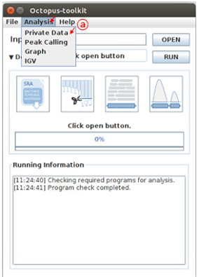
A: Click the Private Data function in the Analysis menu bar.
Select your fastq files and click the Open button.
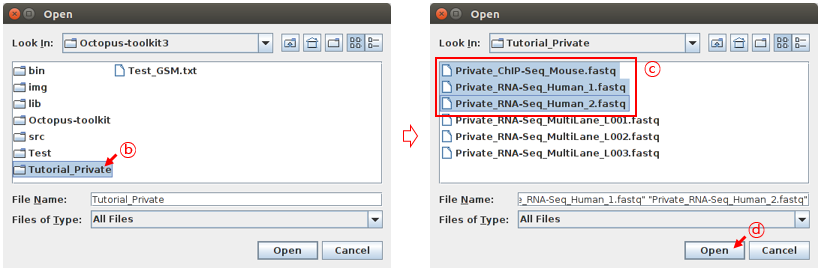
B: select the folderC: Select the filesD: Click the Open button
The following Private Table window will appear.
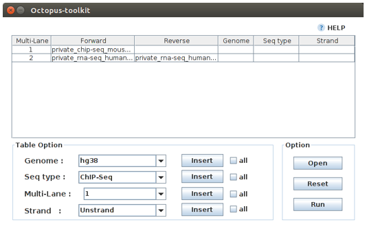
Case 1. Fill in the blank for the 1.Private_ChIP-Seq_Mouse fastq file. Reads in this ChIP-seq file (single-end) should be mapped to the mm10 genome.
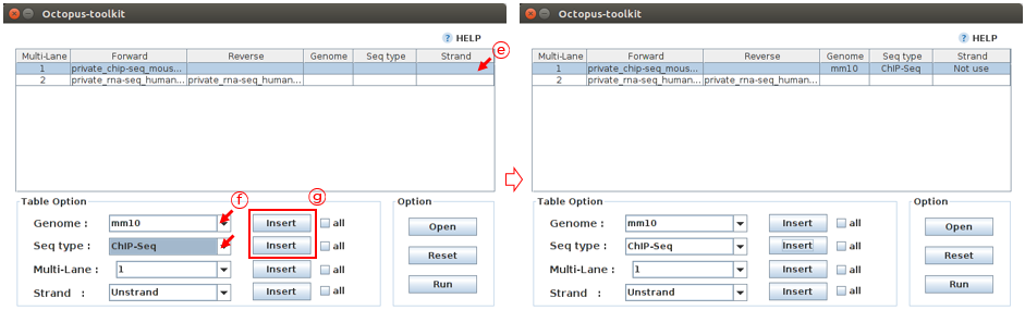
E: Select the Private_ChIP-Seq_Mouse.fastq sample.F: Select appropriate parameters regarding this sample. (Genome :mm10, Seq-Type :ChIP-Seq)G: Click the Insert button
Case 2. Fill in the blank for the 2 and 3.Private_RNA-Seq_Human fastq files. Reads in this RNA-seq files (paired-end, FR-Firststrand) should be mapped to the hg38 genome.
Octopus-toolkit automatically recognizes Paired-End files. The name of the files must be the same and end with the suffix _1.fastq and _2.fastq
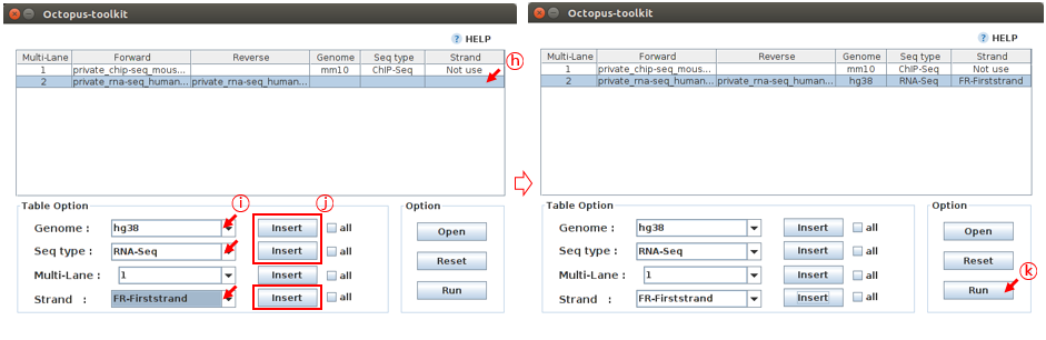
H: Select the Private_RNA-Seq_Human.fastq sample.I: Select information about this sample. (Genome :hg38, Seq-Type :RNA-Seq, Strand :FR-Firststrand)J: Click the Insert buttonK: Click the Run button
The Octopus-toolkit option window will appear. In the Option window, set the parameters for the analysis and click the RUN button to begin the analysis.
L: Click the Run button.
6-4.Private data (Multi-lane)
Note
6-4.Private data (Multi-lane) describes how to process your samples from multe lanes.
| NO | File name | Genome | Seq Type | SE or PE | Strand |
|---|---|---|---|---|---|
| 1 | Private_ChIP-Seq_MultiLane_L001.fastq | hg38 | ChIP-Seq | Single-End | Not use |
| 2 | Private_ChIP-Seq_MultiLane_L002.fastq | hg38 | ChIP-Seq | Single-End | Not use |
| 3 | Private_ChIP-Seq_MultiLane_L003.fastq | hg38 | ChIP-Seq | Single-End | Not use |
First, open the Analysis tab and then, click Private data function.
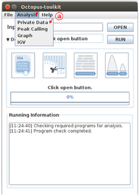
A: Click the Private Data in the Analysis menu bar.
Select your fastq (multi-lane) files and click the Open button.
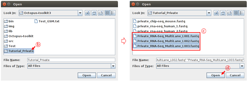
B: select the folderC: Select the filesD: Click the Open button
The following Private Table window will appear.
Case 1. let’s fill in the blank for the Private_ChIP-Seq_MultiLane fastq file. Reads in these ChIP-seq files (single-end) should be mapped to the hg38 genome. Since all samples have the same information, you can use the all button to enter the same information at once.
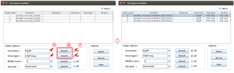
E: Select information about this sample. (Genome :hg38, Seq-Type :ChIP-Seq)F: Click the all buttonG: Click the Insert button
Octopus-toolkit will merge the files with the same number in the Multi-Lane column prior to analysis. Please carefully assign the same number to multi-lane fastq files.
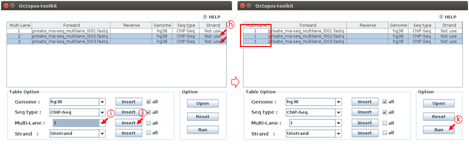
H: Select the Private_RNA-Seq_MultiLane Files.I: Select the number 1 (Multi-Lane)J: Click the Insert buttonK: Click the Run button
The Octopus-toolkit option window will appear. In the Option window, set the parameters for the analysis and click the RUN button to begin the analysis.
L: Click the Run button
6-5.Peak Calling
Note
6-5.Peak Calling describes how to identify peaks (enriched regions by mapped reads) with the Octopus-toolkit output.
You can identify peaks from the output: 6-1 ~ 6-4.
Let’s say you have the following ChIP-seq data.
| NO | Sample name | Input/Control/IgG | Style | Result Path |
|---|---|---|---|---|
| 1 | STAT5A_P6 | Input_P6 | Transcription Factor | Result/GSE48685 |
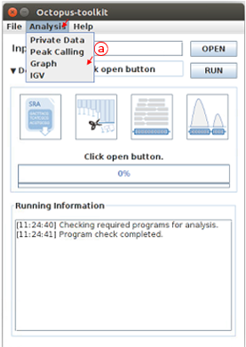
First, open the Analysis tab and then, click the Peak Calling function.
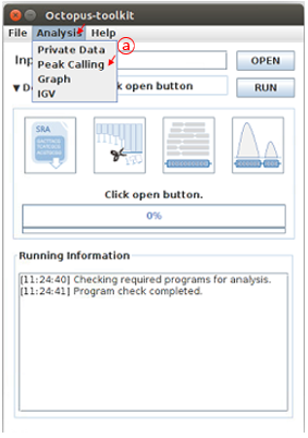
A: Click the Peak Calling in the Analysis menu bar.
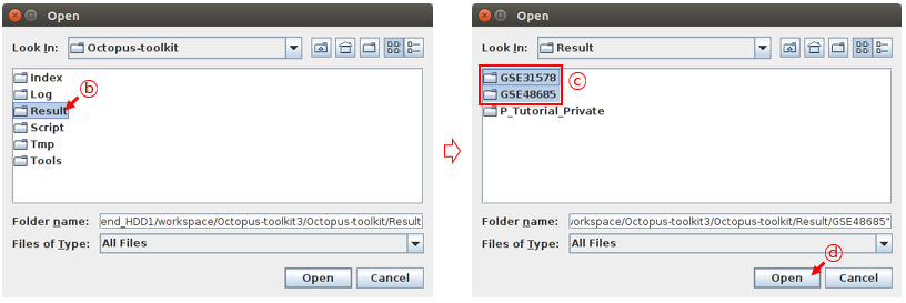
Octopus-toolkit output will be stored in the Result folder. You need to select an appropriate study (GSE directory) in the Result folder. For example, select the GSE48685 directory.
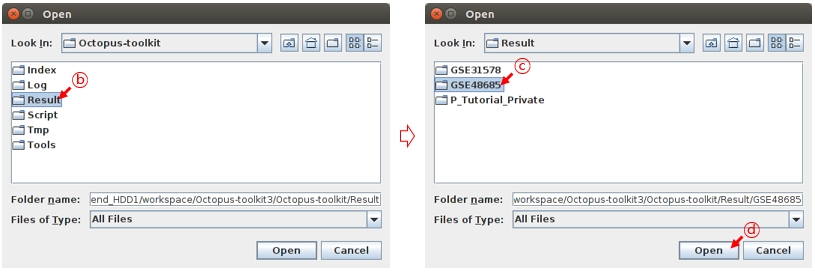
B: Select the Result folder.C: Select the GSE48685 folder.D: Click the Open button.
Once you select an GSE folder (not double click), please click the Open button. Then, the Peak Calling Table will appear.
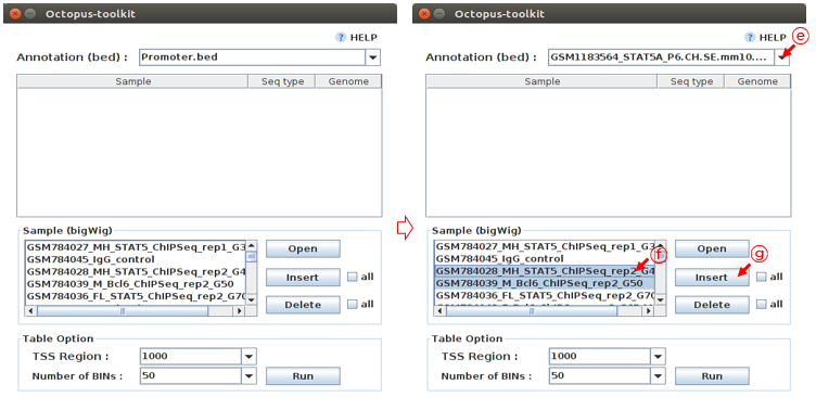
Samples of GSE48685, which were processed by Octopus-toolkit, will appear in the Sample area.
First, you need to add the processed samples to the Peak Calling table using the Insert function.
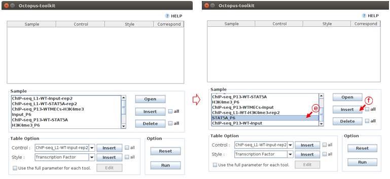
E: Select the STAT5A_P6F: Click the Insert button
Then fill in the blanks for the selected samples using the Table option function. If there is a control (Control) sample to filter out background noise, you also need to add it to the Correspond column.
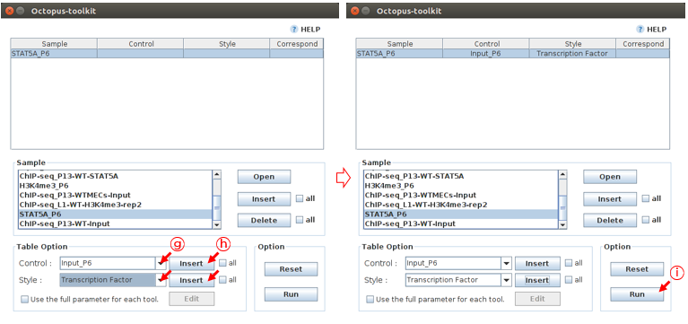
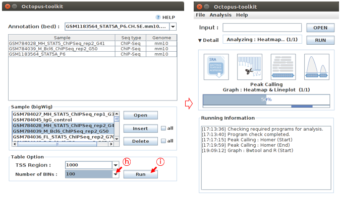
G: Select the information about STAT5A_P6 (Control :Input_P6, Style :Transcription Factor)H: Click the Insert buttonI: Click the Run button
Peak Calling analysis will start according to the Table information.
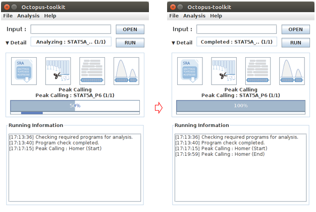
Once completed, you can find the result files (.bed for peaks) in the 05_Analysis directory in the Result/GSE48685 directory.
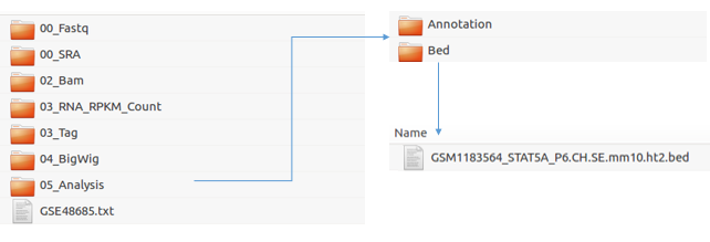
Result Path: Octopus-toolkit/Result/GSE48685
6-6.Graph
Note
6-6.Graph describes how to draw plots with the output: 6-1 ~ 6-5.
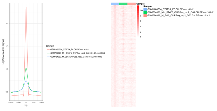
You can draw a heatmap and line plots with a few clicks.
6-6.Graph tutorial describes how to draw plots for multiple outputs. Let say you have the following outputs processed by Octopus-toolkit.
| NO | Sample name | Peak(.bed) |
|---|---|---|
| 1 | STAT5A_P6 | O |
| 2 | M_Bcl6_rep2_G50 | X |
| 3 | MH_STAT5_rep2_G41 | X |
- Option : +-
1000 bpbased on TSS, Bin Size :100
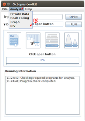
First, open the Analysis tab and then, click the Graph function.
A: Click the Graph in the Analysis menu bar.
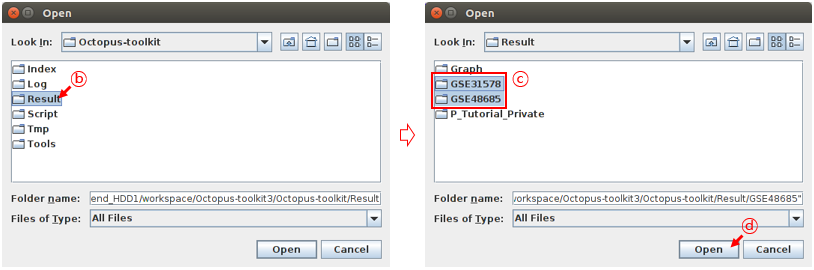
Octopus-toolkit output will be stored in the Result folder. To draw heatmap and plot, you need to select appropriate studies (GSE directories) in the Result folder. For example, select the GSE48685 and GSE31578 directories.
B: Select the Result folder.C: Select the GSE48685 and GSE31578 folders.D: Click the Open button.
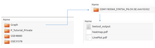
The heatmap and plot will be drawn based on an annotation file (reference). The default annotation file (.bed) contains promoter regions. You can replace it with peak file (.bed) generated by Octopus-toolkit if you perform the peak calling analysis.
E: Select STAT5A_P6_CH.SE.mm10 as the reference.F: Select samples of your interest from the list.G: Click the Insert button.
In the Table option, Adjust TSS region (bp) and Number of BINs (resolution) parameters. Click the Run button to perform the Graph analysis.
H: Select the 1000 in TSS region and 100 in Number of BINsI: Click the Run button
Heatmap and plot will be stored in the Result/Graph folder.
6-7.IGV
Note
6-7.IGV describes how to visualize genomes with data (bigWig files) via IGV.
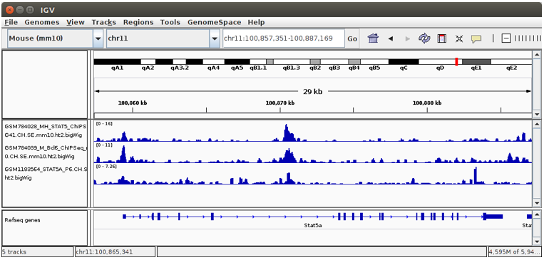
Octopus-toolkit generates bigWig files which can be visualized using Integrative Genomics Viewer(IGV).
First, open the Analysis tab and then, click the IGV function.
A: Click the IGV in the Analysis menu bar.
You need to select appropriate studies (GSE directories) in the Result folder. For example, select the GSE48685 and GSE31578 directories. It will load all bigWig files in the selected directories.
B: Select the Result folder.C: Select the GSE48685 and GSE31578 folders.D: Click the Open button.
Let’s say you select the following samples. You must select an appropriate genome for visualization. Obviously, you cannot load bigWig files from different genomes.
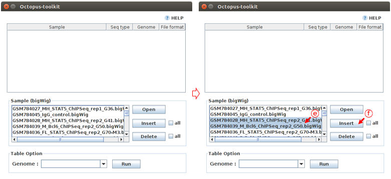
E: Select samples.F: Click the Insert button.
Click the Run button to start the Graph analysis.
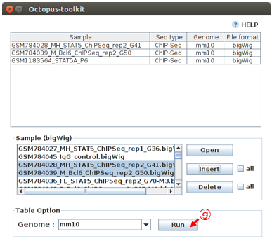
G: Click the Run button.
Depending on the number and size of data, it may take some time to load those files onto the IGV. Please take your time.
6-8.User’s custom adapter sequence(Trimming)
Note
6-8.IGV describes how to use a custom adapter sequence generated by ownself.
Typically, The user uses the adapter sequence provided Trimmomatic. But some users want to use custom adapter sequence generated by ownself.
First, The user should make a custom adapter sequence file. The format of files equals a single or multiple sequence file. (File name extension is .fasta and .fa) (Custom_adapter.fasta)
For more detailed information, please refer to the link below. (Trimmomatic : How to make the adapter fasta)
Second, click the Quality & Trimming button in Octopus-toolkit.
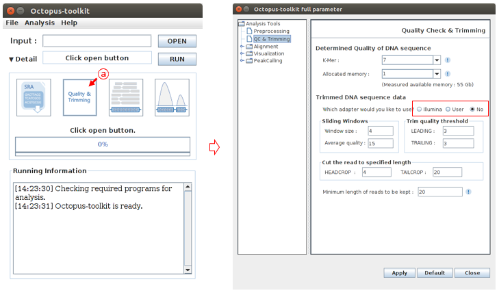
A: Click the Quality & Trimming button.
To open the custom adapter sequence file, Select a User radio button and click the Open button. You need to select your adapter sequence file in your computer.
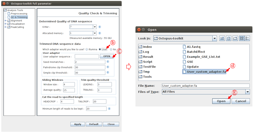
B: Click the User radio button.C: Click the Open button.D: Select the custom adapter sequence file generated by user.E: Click the Open button
Click the Apply button to apply the custom adapter sequence.
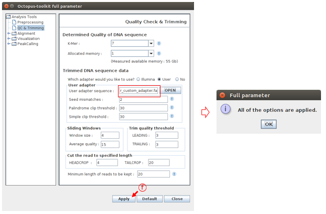
F: Check the Apply button.
6-9.Motif analysis
Note
6-9.Motif analysis describes how to discover de novo and known motif using the output file of Octopus-toolkit : 6-1 ~ 6-5.
Octopus-toolkit is not supporting a motif analysis yet.
The user can analyze de novo and known motif using below command before to be completing development about motif analysis.
We will use a bed format file, which is generated by peak calling in Octopus-toolkit, for discovering motif.
| NO | command | Description |
|---|---|---|
| 1 | Pathway of Octopus-toolkit | /home/user_id/Octopus-toolkit/ |
| 2 | user_id | octopus |
| 3 | Output of Octopus-toolkit | GSE48685 |
| 4 | Input file like bed format file | 05_Analysis/Bed/GSM1183564_STAT5A_P6.CH.SE.mm10.ht2.bed |
| 5 | Genome | mm10 |
The
commandforMotifanalysis:// Add the Homer pathway export Octopus_Homer="/home/user_id/Octopus-toolkit/Tools/Homer/bin" export PATH=$PATH:$Octopus_Homer cd /home/octopus/Octopus-toolkit/Result/GSE48685/ mkdir 06_Motif_output /home/octopus/Octopus-toolkit/Tools/Homer/bin/findMotifsGenome.pl 05_Analysis/Bed/GSM1183564_STAT5A_P6.CH.SE.mm10.ht2.bed mm10 06_Motif_output/
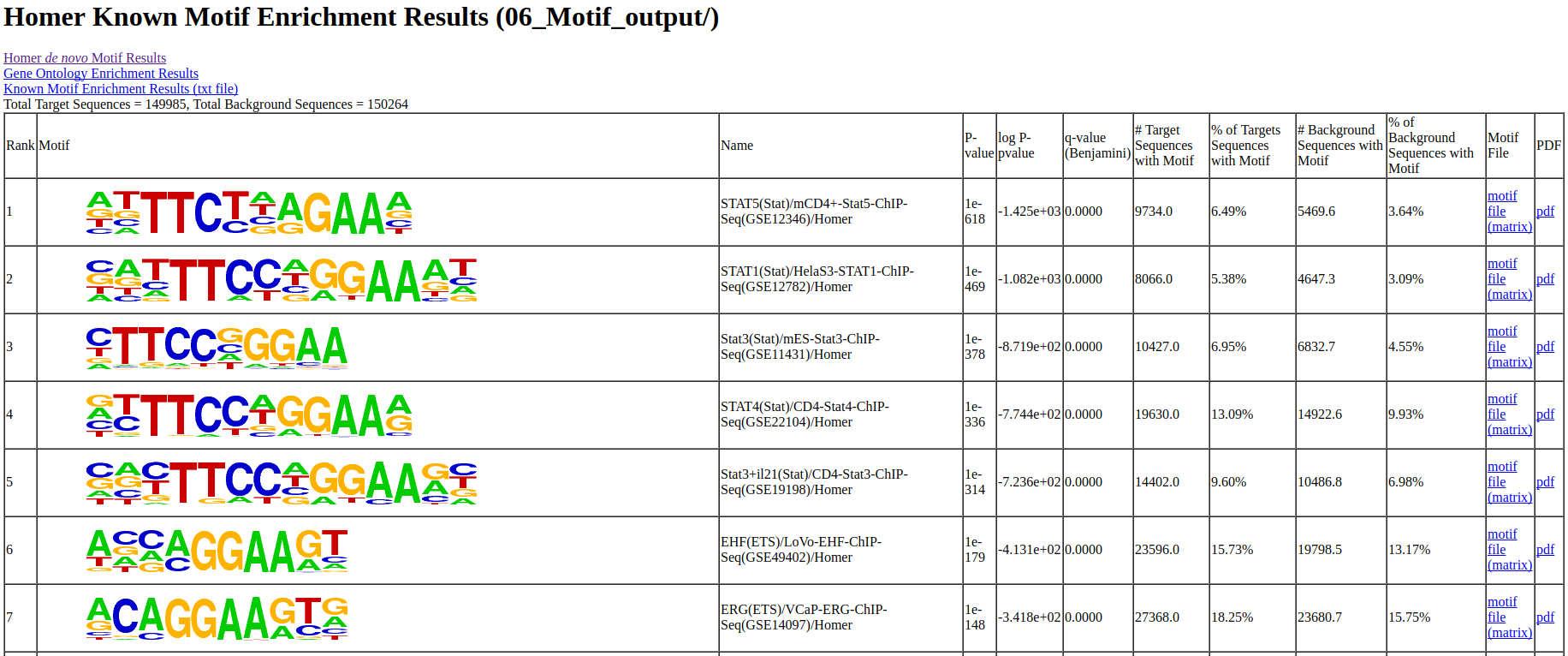
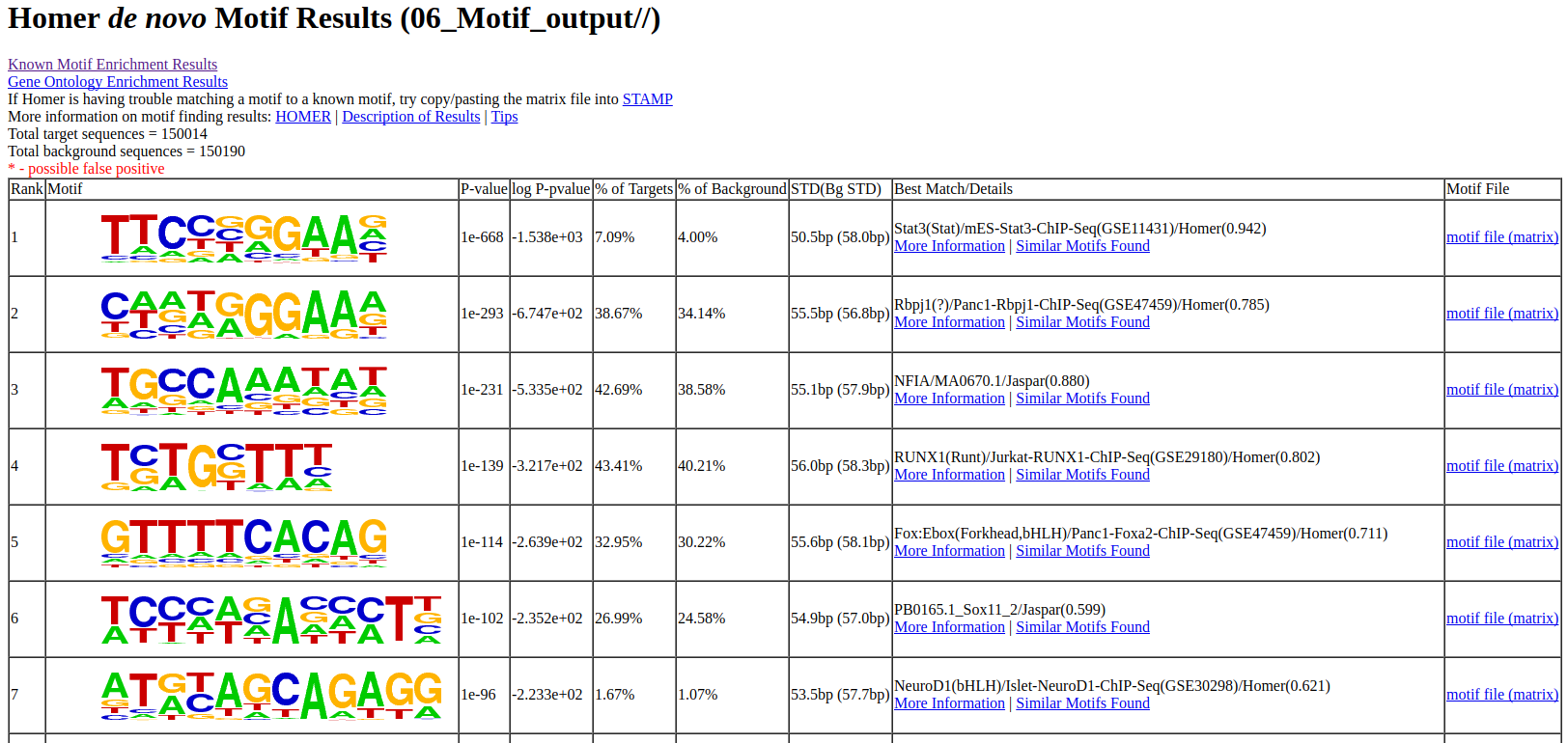
The output of the Motif analysis.
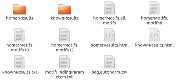
The output of Motif analysis provides a motif’s letter-probability matrix, list of a detected motif, statistical value and best-matched gene symbol.
homerResults.html : De novo Motif
knownResults.html : known Motif