5.User Guide

Octoput-toolkit can analyze a number of publicly available next-generation sequencing (NGS) data in with a single step. In addition, you can also analyze your own data (.fastq) using the same analysis pipeline that is provided by the Octopus-toolkit.

• Supported NGS types : RNA-seq, ChIP-seq, ATAC-seq, DNase-seq, MeDIP-seq, and MNase-seq
• Public data : NGS data released from gene expression omnibus (GEO).
• Private data : NGS data stored in your computer (.fastq or .fastq.gz)

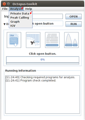
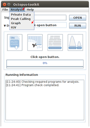
Octopus-toolkit provides several additional functions for further analysis. * Peak Calling : Identification of read enriched regions (.bed) * Drawing Graph : Drawing line plot and heatmap on specified regions (.bed) * Visualization : Explore genome with bigWig files through IGV

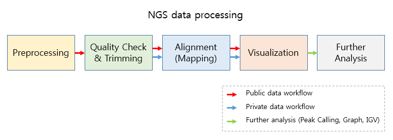
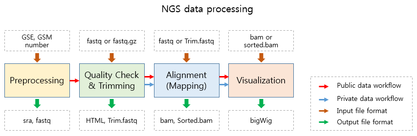
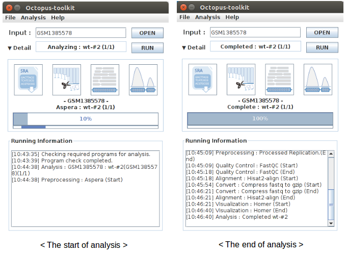
Basically, Octopus-toolkit processes NGS data by the following steps.

• NGS data processing

5-1.3rd party tools used in Octopus-toolkit

Octopus-toolkit utilizes the following 3rd party tools during the process.

NGS Process	Function	3rd party tool	Sub-tools
Preprocessing	Download SRA files from NCBI	Aspera	ascp
	Convert SRA files to Fastq files	SRAToolkit	fastq-dump
Quality check	Quality check for raw data	FastQC	fastqc
Trimming	Trimming for adapter sequence and portions of low-quality reads	Trimmomatic
Alignment	Indexing a reference genome	Hisat2, STAR	hisat2-build, STAR
	Mapping reads to the reference genome	Hisat2, STAR	hisat2-align, STAR
Visualization	Create bigWig files for visualization	Homer	makeTagDirectory,makeUCSCFile,analyzeRepeats
Peak calling	Detect enriched regions by mapped reads	Homer	findPeak, pos2bed,annotatePeaks
Graph	Calculate normalized values from bigWig files	Bwtool	matrix
	Draw the heatmap and line plot	R	pheatmap, ggplot2
IGV	Explore the genome with processed data (bigWig files)	IGV

5-2.Public data

Quick Start

Note

1. Enter a GEO (Gene Expression Omnibus) accession number or click the open button to load a list of GEO accession numbers.
2. Click the Run button.
3. Select appropriate options you want to use.
4. Click the Run button to begin the analysis.

Work flow

To analyze a single or a set of publicly available NGS data from GEO.

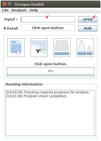
Please enter a single GEO Accession number or open a text file containing GEO Accession numbers.

• Input : GEO Accession number

  GSExxx : Each GSE (study) record is assigned to a single study which contains at least a NGS data (GSM).
  GSMxxx : Each GSM (sample) record is assigned to a single NGS data.
  

• Input : GEO Accession number list (example.list)

1. Enter a single GEO accession number or click the open button to load a list GEO accession numbers.
2. Click the Run button.

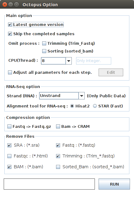
Octopus option

You can change a number of parameters provided by Octopus-toolkit or the integrated tools.

Option	Decription
Latest genome version	Use the latest genome rather than the genome used for the study.
Skip the completed samples	Skip the samples that have already been analyzed.
Omit process	Omit the selected processes such as trimming and sorting steps.
CPU(Thread)	Set the number of CPUs to use.
Adjust all parameters for each step	Change full parameters in each step.
Edit	Open the Full parameter option window.
Strand (RNA)	Set the library strand for RNA-Seq.
Alignment tool for RNA-seq	Set the alignment tool for RNA-seq.
Fastq -> Fastq.gz	Compress Fastq to Fastq.gz.
Bam -> CRAM	Compress Bam to CRAM.
Remove Files	Delete selected intermediate files once each process is completed to save space.

• Latest genome version

Octopus-toolkit can analyze the genomes of Homo sapiens, Mus musculus, Drosophila melanogaster, Saccharomyces cerevisiae, and Canis lupus familaris.

Available analysis genome version

Organism	Genome version
Homo sapiens	hg38, hg19, hg18
Mus musculus	mm10, mm9
Drosophila melanogaster	dm6, dm3
Saccharomyces cerevisiae	sacCer3
Canis lupus familaris	canFam3
Arabidopsis thaliana	tair10
Danio rerio	danRer10
Caenorhabditis elegans	ce11

The latest genome version uses the latest version of the genome for analysis. If you don’t select this option, Octopus-toolkit uses the genome defined by submitter.

• Latest genome (O) : hg38, mm10, dm6, sacCer3, canFam3, tair10, danRer10, ce11
• Latest genome (X) : hg19, mm9, dm3, sacCer3, canFam3, tair10, danRer10, ce11

• Skip the completed samples

While analyzing a number of GSE/GSM data, you can stop the analysis and resume it later.

Octoput-toolkit will skip the samples that have been analyzed completely.

If you have the samples that have been analyzed completely and you want to analyze it again, please do not check this option.

• Omit process

The omit process allows you to skip the trimming step and/or the sorting step. This shortens the anaysis time.

During the trimming process, all reads will be discarded if all of the reads have bad sequencing quality. Octopus-toolkit will analyze the original raw data (.fastq) in this case by skipping the trimming step.

During the sorting process, BAM file will be sorted by using Samtools. In general, many applications uses sorted BAM files. If you are not interested in analyzing the sorted BAM files, you may skip this process.

• CPU(Thread)

You can set the number of CPUs for analysis. (Default : Maximum number of cores depending on your computer)

• Adjust all parameters for each step

You can adjust many parameters for each stop. Check the box and click the Edit button. The parameter window will pop up.

Please refer to the link for details : Full Parameter

• Edit

When you click the Edit button, the parameter window will appear.

• Strand (RNA)

The strand option allows you to choose whether or not to take the stranded information into account. This is only available for stranded-specific RNA-seq.

Octopus-toolkit extracts information from the GEO website when analyzing the public data. However, stranded-specific information of RNA-seq is not well documented. Therefore, this may or may not be applicable depending on the data.

You can select either non-strand library or the strand-specific library such as FR-Firststrand, FR-Secondstrand using this option.

• RNA-Seq alignment tools

You can select an alignment tool to be used during the alignment process for RNA-seq: HISAT2 or STAR.

HISAT2 uses less memory (RAM) than STAR, but STAR is generally faster than HISAT2.

• Fastq->Fastq.gz or Bam->CRAM

You can compress intermediate files to save your disk space.

• Remove Files

Each step creates intermediate files which may or may not be used. If you want to further analyze the processed data, you might want to keep those intermediate files. If not, you can remove intermediate files (up to few hundread gigabytes) by selecting the boxes in Reomve Files window.

Option	Extension	Description
SRA	sra	Compressed raw data downloaded from NCBI. (Sequence Read Archive)
Fastq	fastq or fq	Raw data converted during preprocessing. (A short read sequence file)
Fastqc	html or text	Output generated during Quality Check. (output of FastQC)
Trimming	fastq or fq	Output generated during Trimming. (Trimmed raw file(Fastq))
BAM	bam	Output generated during Alignment. (Mapped read to the genome)
Sorted_Bam	bam	Output generated during Sorting. (Sorted mapped read)

3. Set the paramters and options.
4. Click the Run button to begin the anlaysis.

Run

• Below shows progress bar and status window (GSM1385578).

5-3.Private data

Quick Start

Note

1. Select the analysis tab -> Select the Private Data function in the Menu bar.
2. Select raw files (.fastq) in your computer.
3. Add appropriate information for each sample in the private table.
4. Click the Run button in the private table.

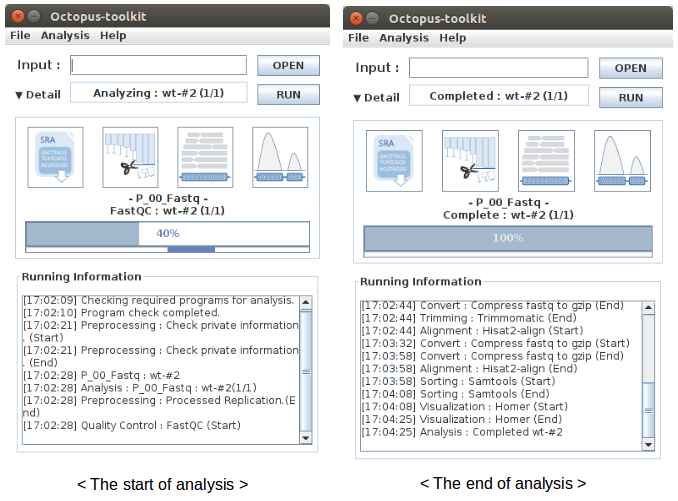
Analyzing your data (private data)

Unlike the public data analysis, private data analysis does not require the converting step (.sra to .fastq).

Input files can be fastq (.fastq or .fq) files or compressed fastq (.fastq.gz or .fq.gz) files.

Files must follow the rules below.

Note

• Raw data : Sample .fastq or Sample .fq
• compressed Raw data : Sample .fastq.gz or Sample .fq.gz
• Single-End data : Sample .fastq (or fq, fastq.gz, fq.gz)
• Paired-End data : Sample _1.fastq, Sample _2.fastq

Octopus-toolkit only loads files that match the above rules.

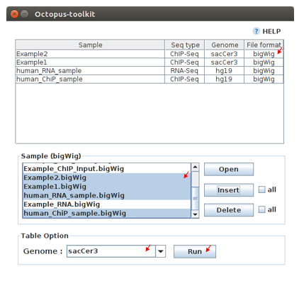
Private table

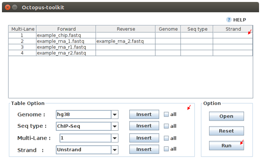
Octopus-toolkit requires appropriate sample information for each file. You need to specify the required information.

If any of the selected files does not appear in the list, please check the file name and format of your files.

You must specify the following information for each sample.

Option	Decription
Genome	Select the genome.
Seq type	Select the experimental type such as ChIP-seq.
Multi-Lane	Set the Multi-lane option.
Strand	Select the strand strategy if applicable.

• Genome

The following genomes are available in the Octopus-toolkit:

Species	Genome version
Homo sapiens	hg38 (Dec.2013, GRCh38), hg19 (Feb.2009,GRCh37), hg18 (Mar.2006 NCBI36)
Mus musculus	mm10 (Dec.2011 GRCm38), mm9 (July.2007 NCBI37)
Drosophila melanogaster	dm6 (Aug.2014 BDGP Release 6+ ISO1 MT), dm3 (Apr.2006 BDGP R5)
Saccharomyces cerevisiae	sacCer3 (Apr.2011 SacCer_Apr2011)
Canis lupus familaris	canFam3 (Sep.2011 Broad CanFam3.1)
Arabidopsis thaliana	tair10
Danio rerio	danRer10 (Sep.2014 GRCz10)
Caenorhabditis elegans	ce11 (Feb.2013 WBcel235)

• Seq type

Octopus-toolkit supports the following experimenatal types: ChIP-Seq, RNA-Seq, MeDIP-Seq, ATAC-Seq, DNase-Seq and MNase-Seq.

• Multi-Lane

A single sample can be obtained from muliple lanes in a sequencing instrument. In this case, files from multe lanes can be merged by setting the same number in the Multi-Lane column.

Multi-lane files generally have the following filenames.

Sample.L001.fastq, Sample.L002.fastq, Sample.L003.fastq ... Sample.L008.fastq

To merge the above files, you must set the number of ‘Multi-Lane columns’ to the same number for each file.

• Strand

This option is to set the library strategy for RNA-seq.

1. Unstranded library : Unstrand (Default)
2. Strand-specific library : FR-Firststrand or FR-secondstrand

Options

Options for private analysis is the same as public data analysis. Please refer to the public data analysis. (Octopus option)

Run

• Snapshots (Private data analysis)

5-4.Peak Calling

Quick Start

Note

1. Select the Analysis tab -> Click the Peak Calling function in the Menu bar.
2. Select the output folder (Result/GSExxxxx) in the Result directory generated by Octopus-toolkit.
3. Add information of each sample in the peak calling table.
4. Click the Run button.

Peak calling anlaysis

The purpose of the peak calling anlaysis is to identify regions enriched by mapped reads.

In order to perform the peak calling analysis, you must have the Octopus-toolkit output folders.

1. Select the Analysis tab -> Click the Peak Calling function in the Menu bar.
2. Select output directories generated by the Octopus-toolkit.

Peak calling table

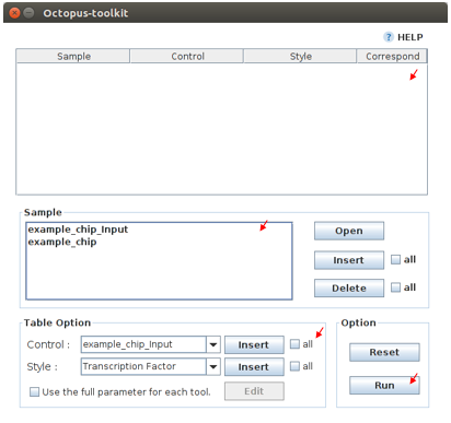
To run the peak calling analysis, please select output folders (Result/GSExxxxx). Then, fill in the blanks using the Table Option functions.

• Control

If available, please select an appropriate control (IgG or input) per sample to filter out the background noise. (Recommended)

• Style

Based on experimental types, you can select a predefined paramter (by HOMER) for the Peak calling process.

option	Seq type	Description
Transcription Factor	ChIP-Seq, DNase-Seq	Peak finding for single contact or focal ChIP-Seq experiments or DNase-Seq.
Histone	ChIP-Seq	Peak finding for broad regions of enrichment found in ChIP-Seq experiments for various histone marks.
DNase	DNase-Seq	Adjusted parameters for DNase-Seq peak finding.
mC	MeDIP-Seq	DNA methylation analysis.

Please select a style option that meets your analysis needs.

3. Add appropriate information for each sample in the private table.
4. Click the Run button in the private table.

5-5.Graph

Quick Start

Note

1. Select the Analysis tab -> Click the Graph function in the Menu bar.
2. Select output folders (Result/GSExxxxx). Multiple output folders can be selected.
3. Set the range of transcription start site (TSS) region and BIN size in the Graph table.
4. Click the Run button.

Start analyzing Graph

The Graph function is to draw average signal pattern on specificed regions which are defined by the user. Signals are extracted from bigWig (normalized to ten million mapped reads) files.

If you would like to draw plots on peaks, you need to complete the peak calling analysis for a sample of your interest.

• Previous steps : Public data or Private data analysis -> Peak Calling.

1. Select the Analysis tab -> Click the Graph function in the Menu bar.
2. Select output folders generated by either Public analysis or Private analysis.

Graph table

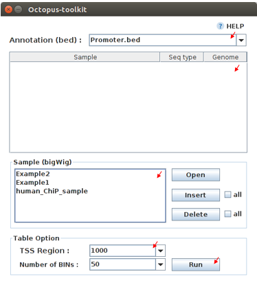
To draw graphs, Octopus-toolkit requires bigWig (signal) files, which are generated by either Public anlaysis or Private analysis.

• bigWig : Output of the Public data or Private data analysis.
• bed : Output of the Peak calling analysis.

Finally, hit the Run button. The output (plots) will be stored in the Graph directory under the Result folder.

• Annotation(bed)

First, select loci (.bed) of your interest from the Annotation (bed) function. Second, select samples (.bigWig) of your interest from the Sample list.

• TSS Region

Third, set appropriate paramters from the Table option. The unit for this option is basepair (bp).

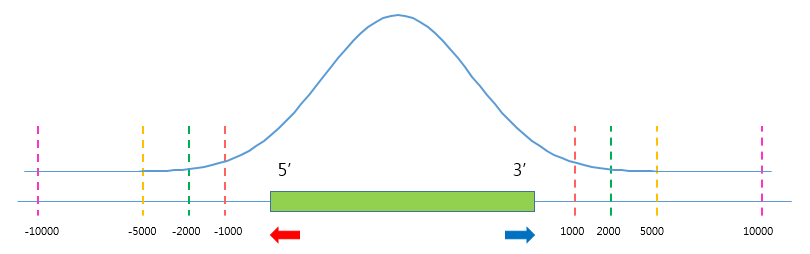
The default ranges of TSS-regions are 1000, 2000, 5000 and 10000 bp.

• Number of BINs

The region selected in the TSS region option is divided into n (number of BINs) BINs

The lager the bin size, the smoother the graph can be drawn.

3. set the TSS region and BIN size in the Graph table.
4. Click the Run button.

5-6.Visualization

Quick Start

Note

1. Select the Analysis tab -> Click the IGV function in the Menu bar.
2. Select output folders (Result/GSExxxxx) of your interest.
3. In the sample window, select samples and then, click the Insert button.
4. Check see if all genomes are the same. Only data in the same genome can be loaded into the IGV.
5. Set the same genome in the Table option.
6. Click the Run button.

Start analyzing IGV

The IGV function is a process of visualizing analyzed data through IGV, a visualization tool.

IGV uses bigWig files.

1. Select the Analysis tab -> Click the IGV function in the Menu bar.
2. Select output folders (Result/GSExxxxx) of your interest.

IGV table

• Genome

Genome option shows the genome of the samples.

3. In the sample window, select samples and then, click the Insert button.
4. Check if all genomes are the same. Only the data in the same genome can be loaded into the IGV.
5. Set the same genome in the Table option.
6. Click the Run button.

Run

• Below shows run screen of IGV.

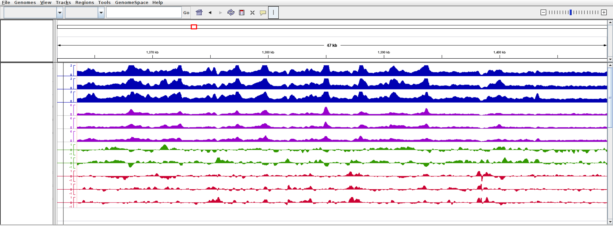
Unlike other tools integrated in Octopus-toolkit, the IGV tool runs separately from the Octopus-toolkit.

5-7.Output (important!)

The output files generated by each process are as follows:

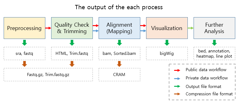
• In the Result folder

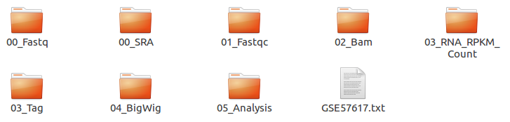
Folder name	Process	File format	Description
00_Fastq	Preprocessing,Trimming	fastq, Trim.fastq	Save the raw file and trimmed file.
00_SRA	Preprocessing	sra	Store the SRA file downloaded from NCBI
01_Fastqc	Quality check	html, txt	Save the result of the Quality check.
02_Bam	Alignment	bam, sorted.bam, bai	Save the Alignment and sorted files.
03_RNA_RPKM_Count	Normalization	RPKM, Count	Save the calculated RPKM and raw read count tables for the RNA-Seq data.
03_Tag	Downstream (motif) analyses by HOMER	Tag folder	Save the Tag folders created by the Homer tool.
04_BigWig	Visualization	bigWig	Save the bigWig files for visualization
05_Analysis	Peak Calling,Annotation	bed, annotation	Save the peak (.bed) and annotation files.
GSE57617.txt	Log file	txt	Sample.txt is a file that stores the analysis status and information.

5-8.File Naming

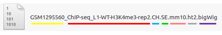
• Yellow : GSM Accession number

  Only applicable for the public data.

• Red : ChIP-Seq_L1-WT-H3K4me3-rep2

  Sample file name (title) defined on the GEO website.

• Blue : Experimental types described below.

Experimental types	Abbreviation	Experimental types	Abbreviation	Experimental types	Abbreviation
ChIP-Seq	CH	RNA-Seq	RN	MeDIP-Seq	ME
ATAC-Seq	AT	DNase-Seq	DN	MNase-Seq	MN

• Green : Sequencing strategy

  SE : Single-End, PE : Paired-End

• Pink : Reference genome

  Reference Genome

• Gray : Alignment tool

  RNA-Seq alignment tools. (ht2 : Hisat2, str: STAR)

• Purple : File extension

  Output Format

5-9.Full Parameters

You can adjust the parameters of 3rd party tools integrated into the Octopus-toolkit.

The 3rd party tools used in Octopus-toolkit : 3rd party tools

Preprocessing

In the preprocessing step, Octopus-toolkit downloads selected NGS data from NCBI and converts the downloaded (.sra) files to FASTQ files. The 3rd party tools used in the preprocessing step are Aspera and SRAToolkit(fastq-dump)

• Transfer rate

  MAX-RATE : MAX transfer rate (Only Integers)

  MIN-RATE : MIN transfer rate (Only Integers)

  Overwrite : Overwrite-Method, Always(Default), Never, Older, Diff

• Convert Sra to Fastq (Filtering)

  MIN-Read Length : Filter by sequence length >= <Value> (Only Integers)

  Aligned or unaligned reads : Dump only aligned sequence or unaligned sequences, NotUse(Default), Both, Aligned, Unaligned

  Quality conversion (offset) : Offset to use for quality conversion, 33(Default), 64

  Dump biological reads(Only) : Dump only biological reads, No(Default)

QC & Trimming

QC & Trimming is the process of assessing the quality of the reads. If bad sequencing quality are detected, portions of low-quality reads are trimmed. The 3rd party tools used in QC & Trimming are FastQC and Trimmomatic.

• Determining the quality of DNA Sequence

  K-Mer : Specifies the length of Kmer to look for in the Kmer content module, Specified Kmer length must be between 2 and 10. Default length is 7 if not specified.

  Allocated memory : Set the momory available on your computer for Quality check. Provides a measure of currently available memory . (Octopus-toolkit option)

• Trimmed DNA sequence data

  Illumina adapt Sequence : Cut adapter and other illumina-specific sequences from the read.

  Seed mismatches : Specifies the maximum mismatch count which will still allow a full match to be performed

  Palindrome clip threshold : Specifies how accurate the match between the two ‘adapter ligated’ reads must be for PE palindrome read alignment.

  Simple clip threshold : Specifies how accurate the match between adapter or any sequence must be against a read.

  Window size : specifies the number of bases to be averaged.

  Average quality : Specifies the average quality required.

  LEADING : Specifies the minimum quality required to keep a base.

  TRAILING : Specifies the minimum quality required to keep a base.

  HEADCROP : The number of bases to keep, from the start of the read.

  TAILCROP : The number of bases to remove from the start of the read.

  Minimum length of reads to be kept : Specifies the minimum length of reads to be kept.

Alignment-Hisat2

Alignment is the process of mapping reads to a reference genome. The 3rd party tool used in Alignment is Hisat2.

• Input

  Skip N read : Skip the first <int> reads/pairs in the input (none)

  Stop after aligning N reads : Stop after first <int> reads/pairs (no limit)

  Trim N bases 5' end : Trim <int> bases from 5’/left end of reads (0)

  Trim N bases 3' end : Trim <int> bases from 3’/right end of reads (0)

• Scoring

  Ambiguous read penalty : Penalty for non-A/C/G/Ts in read/ref

  Mismatch penalty : Max and min penalties for mismatch; lower qual = lower penalty <2,6>

  Soft-Clipping penalty : Max and min penalties for soft-clipping; lower qual = lower penalty <1,2>

  Read gap penalty : Read gap open, extend penalties (5,3)

  Reference gap penalty : Reference gap open, extend penalties (5,3)

• Alignment

  Ignore all quality values : Treat all quality values as 30 in Phred scale (no)

  Do not align reverse of read : Do not align forward (original) version of read (no)

  Do not align forward of read : Do not align reverse-complement version of read (no)

• Spliced alignment

  Do not spliced alignment : Disable spliced alignment

  Canonical : Penalty for a canonical splice site (0)

  Non-canonical : Penalty for a non-canonical splice site (12)

  MIN-Length : Minimum intron length (20)

  MAX-Length : Maximum intron length (500000)

Alignment-STAR

Alignment is the process of mapping reads to a reference genome. The 3rd party tool used in Alignment is STAR (RNA-Seq only).

• Alignment

  AlignIntronMin : Minimum intron size: genomic gap is considered intron if itsnlength>=alignIntronMin, otherwise it is considered as Deletion (21)

  AlignIntronMax : Maximum intron size, if 0, max intron size will be determined byn(2ˆwinBinNbits)*winAnchorDistNbins (0)

  AlignMatesGapMax : Maximum gap between two mates, if 0, max intron gap will be determined by (2ˆwinBinNbits)*winAnchorDistNbins (0)

• Output Filtering

  OutFilterMultimapNmax : int: maximum number of loci the read is allowed to map to. Alignments (all of them) will be output only if the read maps to no more loci than this value. Otherwise no alignments will be output, and the read will be counted as ”mapped to too many loci” in the Log.final.out. (10)

  OutFilterMismatchNmax : int: alignment will be output only if it has no more mismatches than this value. (10)

  OutFilterMismatchNoverLmax : float: alignment will be output only if its ratio of mismatches to mapped length is less than or equal to this value.(0.3)

Visualization-TagDirectory

Visualization-TagDirectory is the process of creating Tag directories. The 3rd party tool used in TagDirectory is Homer.

• Create tag directory

  Fragment-Length : (Set estimated fragment length - given: use read lengths), By default treats the sample as a single read ChIP-Seq experiment

  Maximum tags per bp : Maximum tags per bp, default: no maximum

  Flip the strands of each read : Flip strand of each read, i.e. might want to use with some RNA-seq

  Length of the read to keep : Filter reads with lengths outside this range

Visualization-MakeBigWig

MakeBigWig is the process of creating bigWig files from the Tag directories. The 3rd party tool used in MakeBigWig is Homer.

• Make visualization data

  Size of the bigWig files : Size of file, when gzipped, default: 1e10, i.e. no reduction

  Fragment Length : Approximate fragment length, default: auto

  Resolution : Resolution, in bp, of file, default: 1, avg report average coverage if resolution is larger than 1bp, default: max is reported

  Tags per bp to count : Minimum and maximum tags per bp to count, default: no limit

  Plot negative values : Plot negative values, i.e. for - strand transcription

• Normalization

  Normalize the total number of reads : Total number of tags to normalize experiment to, default: 1e7

  Set the standard length : Expected length of fragment to normalize to [0=off], default: 100

PeakCalling-ChIP-Seq/Histone

PeakCalling is the process of detecting enriched regions (peaks) by mapped reads. The 3rd party tool used in PeakCalling is Homer.

• ChIP-Seq/Histone

  Peak size : Peak size, default: 0

  MIN-Distance : Minimum distance between peaks, default: 0 (peak size x2)

  Genome Size : Set effective mappable genome size, default: 2e9

  Fragment Length : Approximate fragment length, default: auto

  Input Fragment Length : Approximate fragment length of input tags, default: auto

  Tag : Maximum tags per bp to count, 0 = no limit, default: auto

  Input tag : Maximum tags per bp to count in input, 0 = no limit, default: auto

  Tag count to normalize : Tag count to normalize to, default 10000000

  Region Resolution : Extends start/stop coordinates to cover full region considered “enriched” (YES), Resolution number of fractions peaks are divided in when extending ‘regions’, def: 4

PeakCalling-Peak Filter

• Peak Filter

  Fold Enrichment(Input) : Fold enrichment over input tag count, default: 4.0

  Poisson p-value threshold(Input) : Poisson p-value threshold relative to input tag count, default: 0.0001

  Fold Enrichment(Local) : Fold enrichment over local tag count, default: 4.0

  Poisson p-value threshold(Local) : Poisson p-value threshold relative to local tag count, default: 0.0001

  Fold Enrichment(Unique Tag) : Fold enrichment limit of expected unique tag positions, default: 2.0

  Local Size(Local tag) : Region to check for local tag enrichment, default: 10000

  Input Size(Input tag) : Size of region to search for control tags, default: 0

  `False Discovery Rate : False discovery rate, default = 0.001

  Poisson p-value cutoff : Set poisson p-value cutoff, default: 0.001

  Set # of tags : Set # of tags to define a peak, default: 25

  Set # of normalized tags : Set # of normalized tags to define a peak, by default uses 1e7 for norm

PeakCalling-Other analysis

• MethylC-Seq/BS-Seq

  Find Region : Find unmethylated/methylated regions, default: -unmethyC

  Methyl Threshold : Methylation threshold of regions, default: avg methylation/2

  Min cytosine per Methyl : Minimum number of cytosines per methylation peak, default: 6